Non-linear effects and multiplicative interaction terms? A word of caution.

TL;DR-version: if you’re using multiplicative interaction models and the interacted independent variables are correlated, you have to be extra careful to identify even minor non-linearity in main effects.

Interaction effects in various kinds of regression analyses are very common across both the social sciences as well as in, for example, medicine, when we are trying to see whether a main effect varies conditional on some other variable – for example, whether a treatment effect is stronger in men or women, or whether a correlation between two aggregated measures varies between different types of countries.

In an upcoming paper, Hainmueller et al discuss the current best practices when using simple multiplicative interaction effects in regression analysis, and conclude that there are certain endemic problems in how interactions are used that could potentially result in significant interaction terms being artifacts of some violated underlying assumptions. In their paper, they discuss the two problems of interaction effects themselves potentially being non-linear, and of extrapolating the interaction to areas where there are empty cells (as they call it, lack of common support). These two problems are well-known when it comes to simple additive models (avoid fitting a straight line to a clearly curvilinear scatter, and don’t extrapolate the regression line outside of the distribution of the independent variables), but may have been neglected when it comes to interactions.

This lead me to think a bit about a related problem that I’ve occasionally encountered: estimating interaction models when failing to account for a main unconditional effect that is non-linear. It is often argued that minor cases of non-linear main effects are generally not an issue, and that linear OLS (particularly with heteroskedasticity-consistent standard errors) is fairly robust even in these cases. While linear OLS will indeed generally find the correct sign of an association even when it is diminishing, adding multiplicative interactions in this situation can be highly problematic.

The essence of the problem is the following: if a moderating variable is correlated with an independent variable that is non-linearly related to the dependent variable, then trying to fit a linear interacted model may result in an entirely spurious significant interaction effect. To add insult to injury, this is an issue that becomes worse the larger your sample is.

Though this is seemingly a rather intuitive problem, I’ve never seen it mentioned. I flipped through a number of textbooks in quantitative methods and econometrics that were laying around the office, and of about ten books that covered how to use multiplicative interactions, none issued any warning about this. (EDIT: an attentive reader directed my attention to section 5.6 in another paper by Hainmueller & Hazlett, that touches on this issue).

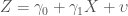
Consider a couple of typical regression equations. Let’s assume that the correct specifications for Y and Z are the following:

$Y=\beta_{0}+\beta_{1}X+\beta_{2}X^{2}+\epsilon$

and

$Z=\gamma_{0}+\gamma_{1} X + \upsilon$ .

A typical multiplicative interaction model for Y, X and Z would look like this:

$Y=\delta_{0}+\delta_{1}X + \delta_{2}Z + \delta_{3}X\times Z+\psi$ .

The “correct” version is that Y is a function of a second-degree polynomial of X, and Z is a linear function of X. Z is thus related to Y only insofar as it correlates with X – the definition of spurious. Since Z tends to be higher when X is higher, and the rate of change in Y is different when X is higher, the rate of change in Y will also be different, on average, when Z is higher. For simplicity we disregard the error terms and the intercepts and look at the two simple equations 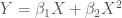$Y=\beta_{1}X+\beta_{2}X^{2}$ and $Z=\gamma_{1} X$ . If we fit the equation $Y=\delta_{1}X+\delta_{2}Z+\delta_{3}X\times Z$ , some simple substitution and rearrangement reveals that the interaction term turns into $\delta_{3}\gamma_{1} X^{2}$ and thus actually captures the product of the true square coefficient and the correlation between X and Z. And as usual – the larger N, the smaller the standard errors, and the higher the risk of spuriously getting significant interactions. [1]

To see how this turns out in practice, I generated a simple dataset of 100 observations from the following two functions:

$Y=3X - 0.01 X^{2} + e$

where $e \thicksim \mathcal{N}(0,15)$ , and

$Z=X+u$

where $u \thicksim \mathcal{N}(0,10)$ . X was uniformly distributed between 1 and 100. The relationship between X and Y that results from this data generating process looks like this:

scatteryx

This relationship is visibly very slightly curvilinear, but it is hardly dramatic – any researcher would be forgiven for deeming it approximately linear and choosing to fit a straight line. In the simple bivariate case, that would be completely fine, and yet, with an interaction, everything breaks down. The table below summarizes the relevant regression models.

table1

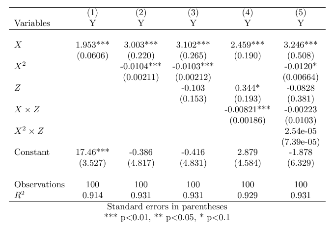
As we can see, the interaction model in column 4 performs just as good in terms of goodness of fit as the correctly specified model in column 2, and finds two completely spurious coefficients: both for Z as such (not to be interpreted as an unconditional effect, of course), and for an interaction between X and Z. This, as noted, is a direct consequence of failing to account for the slight curvilinearity of the relationship between X and Y. Despite the fact that the slowly diminishing effect of X is just barely visible upon ocular inspection, it wreaks complete havoc on our results when using an interaction term. When using the correctly specified non-linear model and controlling for the interaction with Z in model 5, we again get the “correct” results.

The above example is driven by a high level of correlation between X and Z, that is granted, and the degree of statistical fit obtained is unlikely to turn up in the real world. So is this really a problem in practice? I think it could be. Let’s take an obvious real-world example as well. Let’s consider the relationship between GDP per Capita and life expectancy. I will use data on life expectancy and GDP per Capita from the World Development Indicators from 2012 . As a conceivable moderator, I will use the level of democracy, as operationalized in the revised combined Polity IV and Freedom House indices (fh_ipolity2 in the QoG Standard dataset). Consider the plots below of the relationship between GDP per Capita and life expectancy. This is a highly diminishing relationship:

gdplifexp

There are different ways of dealing with this type of relationship, but here I will use what is arguably the standard solution in this case: logging the independent variable. The scatterplot below shows a much better linear fit after such a transformation.

Now, what happens when we include our moderator, democracy? We have strong prior suspicions that democracies tend to be richer, and this turns out to apply to this data: pearson’s r between the two is roughly 0.4. Here is a regression table with the relevant models.

Voila. Model 5, that fails to account for the curvilinear relationship between wealth and life expectancy, spuriously finds that democracy is a negative moderator! Now we just need to find a cool post-hoc explanation for this (wealth is bad for us in democracies because we’re free to spend it all on junk food) and we’re good to go. I can already see the headlines. Meanwhile, model 6, with the transformed GDP per Capita that takes its non-linear effect into account, has significant coefficients for neither democracy, nor the interaction term (although in this case, multicollinearity becomes a problem instead). (You may ask – would someone really fail to account for this in reality? Consider this paper, that has been cited 210 times according to Google Scholar. The main result turns out to be completely an artifact of not correctly specifying GDP per Capita).

The general guideline thus should be something like this: if the main treatment effect is really even slightly non-linear, and the proposed moderator is correlated with the main independent variable, accounting for the non-linear main effect is crucial when fitting an interaction, and arguably much more important than in a model without such an interaction.

More specifically, the consequence of not doing so depends on what type of non-linear main effect we have, and the sign of the relationship between the independent variables. If the main effect is diminishing, and the moderator is positively correlated with the treatment, then a linear multiplicative interaction model will spuriously find a negative interaction. If the main effect is diminishing and the moderator is negatively correlated with the treatment, then a linear multiplicative interaction model will spuriously find a positive interaction. Vice versa applies for a main effect that is increasing.

1. One may add that the converse of this problem arises when we are attempting to fit a non-linear function to an effect that is truly interactive. This perhaps deserves a treatment of its own.